Chapter 3 Complex ANOVA and Multiple Linear Regression
In the One-Way ANOVA and simple linear regression models, there was only one variable - categorical for ANOVA and continuous for simple linear regression - to explain and predict our target variable. Rarely do we believe that only a single variable will suffice in predicting a variable of interest. Here in this Chapter we will generalize these models to the \(n\)-Way ANOVA and multiple linear regression models. These models contain multiple sets of variables to explain and predict our target variable.
This Chapter aims to answer the following questions:
- How do we include multiple variables in ANOVA?
- Exploration
- Assumptions
- Predictions
- What is an interaction between two predictor variables?
- Interpretation
- Evaluation
- Within Category Effects
- What is blocking in ANOVA?
- Nuisance Factors
- Differences Between Blocking and Two-Way ANOVA
- How do we include multiple variables in regression?
- Model Structure
- Global & Local Inference
- Assumptions
- Adjusted \(R^2\)
- Categorical Variables in Regression
3.1 Two-Way ANOVA
In the One-Way ANOVA model, we used a single categorical predictor variable with \(k\) levels to predict our continuous target variable. Now we will generalize this model to include \(n\) categorical variables that each have different numbers of levels (\(k_1, k_2, ..., k_n\)).
3.1.1 Exploration
Let’s use the basic example of two categorical predictor variables in a Two-Way ANOVA. Previously, we talked about using heating quality as a factor to explain and predict sale price of homes in Ames, Iowa. Now, we also consider whether the home has central air. Although similar in nature, these two factors potentially provide important, unique pieces of information about the home. Similar to previous data science problems, let us first explore our variables and their potential relationships.
Now that we have two variables that we will use to explain and predict sale price, here are some summary statistics (mean, standard deviation, minimum, and maximum) for each combination of category. We will use the group_by function on both predictor variables of interest to split the data and then the summarise function to calculate the metrics we are interested in.
3.1.1.1 R code:
train %>%
  group_by(Heating_QC, Central_Air) %>%
  dplyr::summarise(mean = mean(Sale_Price),
            sd = sd(Sale_Price),
            max = max(Sale_Price),
            min = min(Sale_Price),
            n = n())
## `summarise()` has grouped output by 'Heating_QC'. You can override using the
## `.groups` argument.## # A tibble: 10 × 7
## # Groups: Heating_QC [5]
## Heating_QC Central_Air mean sd max min n
## <ord> <fct> <dbl> <dbl> <int> <int> <int>
## 1 Poor N 50050 52255. 87000 13100 2
## 2 Poor Y 107000 NA 107000 107000 1
## 3 Fair N 84748. 28267. 158000 37900 29
## 4 Fair Y 145165. 38624. 230000 50000 36
## 5 Typical N 103469. 34663. 209500 12789 82
## 6 Typical Y 142003. 39657. 375000 60000 527
## 7 Good N 110811. 38455. 214500 59000 23
## 8 Good Y 160113. 54158. 415000 52000 318
## 9 Excellent N 115062. 33271. 184900 64000 11
## 10 Excellent Y 216401. 88518. 745000 58500 1022We can already see above that there appears to be some differences in average sale price across the categories overall. Within each grouping of heating quality, homes with central air appear to have a higher sale price than homes without. Also, similar to before, homes with higher heating quality appear to have higher sale prices compared to homes with lower heating quality. Careful about samepl size in these situations though!
We also see these relationships in the bar chart in Figure 3.1.
CA_heat <- train %>%
  group_by(Heating_QC, Central_Air) %>%
  dplyr::summarise(mean = mean(Sale_Price),
            sd = sd(Sale_Price),
            max = max(Sale_Price),
            min = min(Sale_Price),
            n = n())
## `summarise()` has grouped output by 'Heating_QC'. You can override using the
## `.groups` argument.ggplot(data = CA_heat, aes(x = Heating_QC, y = mean/1000, fill = Central_Air)) +
geom_bar(stat = "identity", position = position_dodge()) +
labs(y = "Sales Price (Thousands $)", x = "Heating Quality Category") +
scale_fill_brewer(palette = "Paired") +
theme_minimal()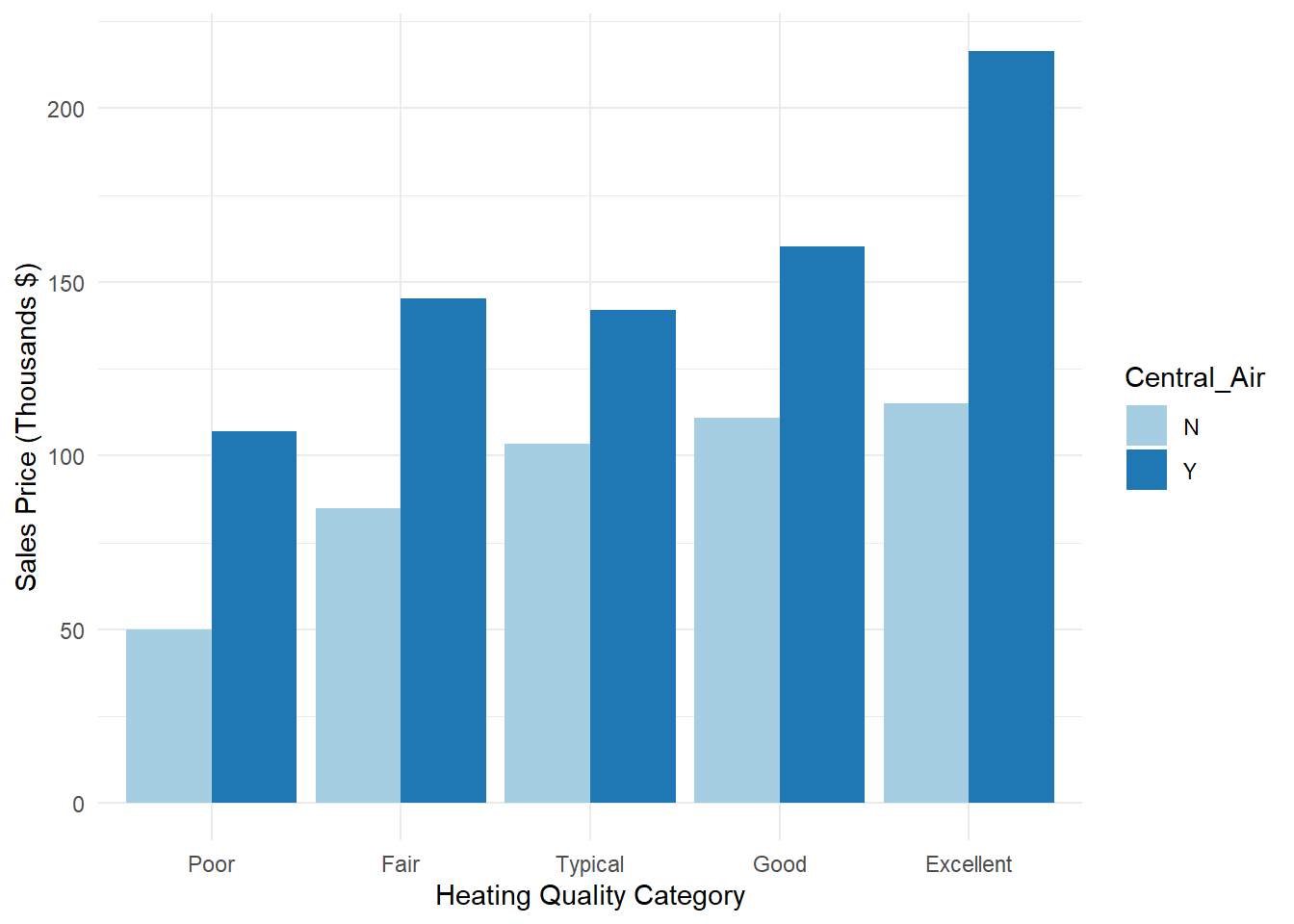
Figure 3.1: Distribution of Variables Heating_QC and Central_Air
As before, visually looking at bar charts and mean calculations only goes so far. We need to statistically be sure of any differences that exist between average sale price in categories.
3.1.2 Model
We are going to do this with the same approach as in the One-Way ANOVA, just with more variables as shown in the following equation:
\[ Y_{ijk} = \mu + \alpha_i + \beta_j + \varepsilon_{ijk} \] where \(\mu\) is the average baseline sales price of a home in Ames, Iowa, \(\alpha_i\) is the variable representing the impacts of the levels of heating quality, and \(\beta_j\) is the variable representing the impacts of the levels of central air. As mentioned previously, the unexplained error in this model is represented as \(\varepsilon_{ijk}\).
The same F test approach is also used, just for each one of the variables. Each variable’s test has a null hypothesis assuming all categories have the same mean. The alternative for each test is that at least one category’s mean is different.
Let’s view the results of the aov function.
##               Df    Sum Sq   Mean Sq F value   Pr(>F)
## Heating_QC     4 2.891e+12 7.228e+11  147.60  < 2e-16 ***
## Central_Air    1 2.903e+11 2.903e+11   59.28 2.11e-14 ***
## Residuals   2045 1.002e+13 4.897e+09
## ---
## Signif. codes:  0 '***' 0.001 '**' 0.01 '*' 0.05 '.' 0.1 ' ' 1
From the above results, we have low p-values for each of the variables’ F test. Heating quality had 4 degrees of freedom, derived from the 5 categories \((4 = 5-1)\). Similarly, central air’s 2 categories produce 1 \((= 2-1)\) degree of freedom. The F values are calculated the exact same way as described before with the mean square for each variable divided by the mean square error. Based on these tests, at least one category in each variable is statistically different than the rest.
3.1.3 Post-Hoc Testing
As with the One-Way ANOVA, the next logical question is which of these categories is different. We will use the same post-hoc tests as before with the TukeyHSD function.
## Tukey multiple comparisons of means
## 95% family-wise confidence level
##
## Fit: aov(formula = Sale_Price ~ Heating_QC + Central_Air, data = train)
##
## $Heating_QC
## diff lwr upr p adj
## Fair-Poor 49176.42 -63650.448 162003.29 0.7571980
## Typical-Poor 67781.01 -42800.320 178362.35 0.4506761
## Good-Poor 87753.89 -23040.253 198548.03 0.1945181
## Excellent-Poor 146288.89 35818.859 256758.92 0.0028361
## Typical-Fair 18604.59 -6326.425 43535.61 0.2484556
## Good-Fair 38577.47 12718.894 64436.04 0.0004622
## Excellent-Fair 97112.47 72679.867 121545.07 0.0000000
## Good-Typical 19972.87 7050.230 32895.52 0.0002470
## Excellent-Typical 78507.88 68746.678 88269.07 0.0000000
## Excellent-Good 58535.00 46602.229 70467.78 0.0000000
##
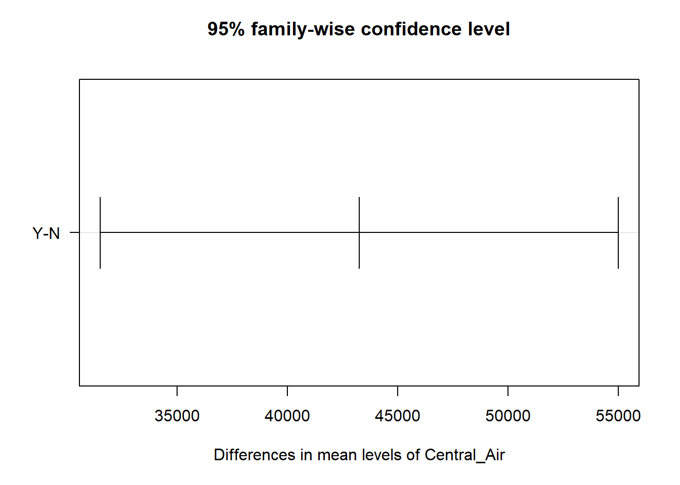
## $Central_Air
## diff lwr upr p adj
## Y-N 43256.57 31508.27 55004.87 0

Starting with the variable for central air, we can see there is a statistical difference between the two categories. This is the exact same result as the overall F test for the variable since there are only two categories. For the heating quality variable, we can see some categories are different from each other, while others are not. Noticeably, the combination of poor with fair, good, and typical categories are not statistically different. Notice also the different widths of these confidence intervals do to the different combinations of sample sizes for the categories being tested.
3.1.4 Python Code
Exploring the data:
summary = (
    train
    .groupby(['Heating_QC', 'Central_Air'])
    .agg(
        mean=('Sale_Price', 'mean'),
        sd=('Sale_Price', 'std'),
        max=('Sale_Price', 'max'),
        min=('Sale_Price', 'min'),
        n=('Sale_Price', 'count')
    )
    .reset_index()
)

print(summary)
## Heating_QC Central_Air mean sd max min n
## 0 Excellent N 112975.000000 36635.766336 184900 64000 13
## 1 Excellent Y 218809.105960 87247.973506 755000 65000 1057
## 2 Fair N 85862.068966 25543.917557 158000 39300 29
## 3 Fair Y 150940.257143 39913.408794 235000 50000 35
## 4 Good N 107186.111111 33810.126422 214500 59000 18
## 5 Good Y 157455.063291 54425.088131 415000 50138 316
## 6 Poor N 50050.000000 52255.191130 87000 13100 2
## 7 Poor Y 107000.000000 NaN 107000 107000 1
## 8 Typical N 102143.342105 43069.612095 265979 12789 76
## 9 Typical Y 145896.166667 42814.810603 375000 70000 504Graph:
p = (
  ggplot(summary, aes(x = "Heating_QC", y = "mean",  fill="Central_Air")) +
  geom_bar(stat = "identity", position = position_dodge()) +
  labs(y = "Sales Price (Thousands $)", x = "Heating Quality Category")  +
  theme_minimal()
    )

p.show()
Two-way ANOVA model
import statsmodels.formula.api as smf
import statsmodels.api as sm


model = smf.ols("Sale_Price ~ C(Heating_QC) + C(Central_Air)", data = train).fit()
model.summary()| Dep. Variable: | Sale_Price | R-squared: | 0.240 |
|---|---|---|---|
| Model: | OLS | Adj. R-squared: | 0.239 |
| Method: | Least Squares | F-statistic: | 129.5 |
| Date: | Tue, 17 Jun 2025 | Prob (F-statistic): | 2.07e-119 |
| Time: | 13:39:04 | Log-Likelihood: | -25806. |
| No. Observations: | 2051 | AIC: | 5.162e+04 |
| Df Residuals: | 2045 | BIC: | 5.166e+04 |
| Df Model: | 5 | ||
| Covariance Type: | nonrobust |
| coef | std err | t | P>|t| | [0.025 | 0.975] | |
|---|---|---|---|---|---|---|
| Intercept | 1.633e+05 | 6920.153 | 23.594 | 0.000 | 1.5e+05 | 1.77e+05 |
| C(Heating_QC)[T.Fair] | -7.185e+04 | 9544.896 | -7.528 | 0.000 | -9.06e+04 | -5.31e+04 |
| C(Heating_QC)[T.Good] | -6.048e+04 | 4432.503 | -13.646 | 0.000 | -6.92e+04 | -5.18e+04 |
| C(Heating_QC)[T.Poor] | -1.125e+05 | 4.1e+04 | -2.743 | 0.006 | -1.93e+05 | -3.21e+04 |
| C(Heating_QC)[T.Typical] | -7.083e+04 | 3724.285 | -19.019 | 0.000 | -7.81e+04 | -6.35e+04 |
| C(Central_Air)[T.Y] | 5.492e+04 | 6656.049 | 8.251 | 0.000 | 4.19e+04 | 6.8e+04 |
| Omnibus: | 816.668 | Durbin-Watson: | 2.013 |
|---|---|---|---|
| Prob(Omnibus): | 0.000 | Jarque-Bera (JB): | 4816.450 |
| Skew: | 1.775 | Prob(JB): | 0.00 |
| Kurtosis: | 9.615 | Cond. No. | 37.3 |
Notes:
[1] Standard Errors assume that the covariance matrix of the errors is correctly specified.
##                       sum_sq      df           F        PR(>F)
## C(Heating_QC)   2.216871e+12     4.0  111.257391  6.745663e-86
## C(Central_Air)  3.390960e+11     1.0   68.072407  2.788148e-16
## Residual        1.018697e+13  2045.0         NaN           NaN
Post-hoc testing
from statsmodels.stats.multicomp import pairwise_tukeyhsd

# Tukey's HSD for Heating_QC
tukey_heating = pairwise_tukeyhsd(endog=train['Sale_Price'],
                                  groups=train['Heating_QC'],
                                  alpha=0.05)
print(tukey_heating)
## Multiple Comparison of Means - Tukey HSD, FWER=0.05
## =====================================================================
## group1 group2 meandiff p-adj lower upper reject
## ---------------------------------------------------------------------
## Excellent Fair -96071.5679 0.0 -121271.5851 -70871.5507 True
## Excellent Good -62777.3129 0.0 -75051.5531 -50503.0728 True
## Excellent Poor -148489.9377 0.0032 -261710.0367 -35269.8387 True
## Excellent Typical -77360.2331 0.0 -87457.6961 -67262.7701 True
## Fair Good 33294.255 0.0061 6573.1446 60015.3654 True
## Fair Poor -52418.3698 0.7296 -168099.6197 63262.8802 False
## Fair Typical 18711.3348 0.2758 -7082.4538 44505.1234 False
## Good Poor -85712.6248 0.2378 -199280.9641 27855.7146 False
## Good Typical -14582.9202 0.0258 -28034.1518 -1131.6885 True
## Poor Typical 71129.7046 0.4259 -42224.0315 184483.4407 False
## ---------------------------------------------------------------------# Tukey's HSD for Central_Air
tukey_air = pairwise_tukeyhsd(endog=train['Sale_Price'],
groups=train['Central_Air'],
alpha=0.05)
print(tukey_air)## Multiple Comparison of Means - Tukey HSD, FWER=0.05
## ============================================================
## group1 group2 meandiff p-adj lower upper reject
## ------------------------------------------------------------
## N Y 88519.3896 0.0 75070.1553 101968.6238 True
## ------------------------------------------------------------3.2 Two-Way ANOVA with Interactions
What if the relationship between a predictor and target variable changed depending on the value of another predictor variable? For our example, we would say that the average difference in sales price between having central air and not having central changed depending on what level of heating quality the home had. In the bar chart in Figure 3.1, a potential interaction effect is displayed when the differences between the two bars within each heating category is different across heating category. If the difference, was the same, then there is no interaction present. In other words, no matter the heating quality rating of the home, the average difference in sales price between having central air and not having central air is the same.
This interaction model is represented as follows:
\[ Y_{ijk} = \mu + \alpha_i + \beta_j + (\alpha \beta)_{ij} + \varepsilon_{ijk} \]
with the interaction effect, \((\alpha \beta)_{ij}\), as the multiplication of the two variables involved in the interaction. Interactions can occur between more than two variables as well. Interactions are good to evaluate as they can mask the effects of individual variables. For example, imagine a hypothetical example as shown in Figure 3.2 where the impact of having central air is opposite depending on which category of heating quality you have.
3.2.0.1 R code:
fake_HQ <- c("Poor", "Poor", "Excellent", "Excellent")
fake_CA <- c("N", "Y", "N", "Y")
fake_mean <- c(100, 150, 150, 100)

fake_df <- as.data.frame(cbind(fake_HQ, fake_CA, fake_mean))ggplot(data = fake_df, aes(x = fake_HQ, y = as.numeric(fake_mean), fill = fake_CA)) +
geom_bar(stat = "identity", position = position_dodge()) +
labs(y = "Fake Sales Price (Thousands $)", x = "Fake Heating Quality Category") +
scale_fill_brewer(palette = "Paired") +
theme_minimal()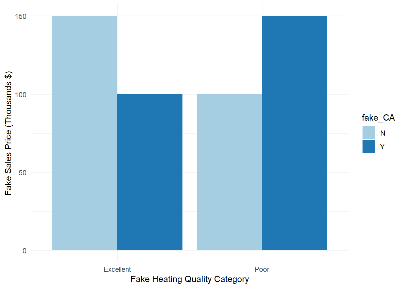
Figure 3.2: Distribution of Variables Heating_QC and Central_Air
If you were to only look at the average sales price across heating quality, you would notice no difference between the two groups (average for both heating categories is 125). However, when the interaction is accounted for, you can clearly see in the bar heights that sales price is different depending on the value of central air.
Let’s evaluate the interaction term in our actual data. To do so, we just incorporate the multiplication of the two variables in the model statement by using the formula Sale_Price ~ Heating_QC + Central_Air + Heating_QC:Central_Air. You could also use the shorthand version of this by using the formula Sale_Price ~ Heating_QC*Central_Air. The * will include both main effects (the individual variables) and the interaction between them.
##                          Df    Sum Sq   Mean Sq F value   Pr(>F)
## Heating_QC                4 2.891e+12 7.228e+11 147.897  < 2e-16 ***
## Central_Air               1 2.903e+11 2.903e+11  59.403 1.99e-14 ***
## Heating_QC:Central_Air    4 3.972e+10 9.930e+09   2.032   0.0875 .
## Residuals              2041 9.975e+12 4.887e+09
## ---
## Signif. codes:  0 '***' 0.001 '**' 0.01 '*' 0.05 '.' 0.1 ' ' 1
As seen by the output above, the interaction effect between heating quality and central air is not significant at the 0.05 level. Again, this implies that the average difference in sale price of the home between having central air and not does not differ depending on which category of heating quality the home belongs to. If our interaction was significant (say a 0.02 p-value instead) then we would keep it in our model, but here we would remove the interaction term from our model and rerun the analysis.
3.2.1 Post-Hoc Testing
Post-hoc tests are also available for interaction models as well to determine where the statistical differences exist in all the combinations of possible categories. We evaluate these post-hoc tests using the same TukeyHSD function and its corresponding plot element.
##   Tukey multiple comparisons of means
##     95% family-wise confidence level
##
## Fit: aov(formula = Sale_Price ~ Heating_QC * Central_Air, data = train)
##
## $Heating_QC
##                        diff        lwr       upr     p adj
## Fair-Poor          49176.42 -63536.973 161889.81 0.7565086
## Typical-Poor       67781.01 -42689.104 178251.13 0.4496163
## Good-Poor          87753.89 -22928.822 198436.60 0.1936558
## Excellent-Poor    146288.89  35929.963 256647.82 0.0027979
## Typical-Fair       18604.59  -6301.351  43510.54 0.2474998
## Good-Fair          38577.47  12744.901  64410.03 0.0004543
## Excellent-Fair     97112.47  72704.440 121520.50 0.0000000
## Good-Typical       19972.87   7063.227  32882.52 0.0002425
## Excellent-Typical  78507.88  68756.495  88259.26 0.0000000
## Excellent-Good     58535.00  46614.230  70455.77 0.0000000
##
## $Central_Air
##         diff      lwr      upr p adj
## Y-N 43256.57 31520.09 54993.05     0
##
## $`Heating_QC:Central_Air`
##                               diff         lwr       upr     p adj
## Fair:N-Poor:N            34698.276 -127178.615 196575.17 0.9996249
## Typical:N-Poor:N         53419.220 -105046.645 211885.08 0.9876643
## Good:N-Poor:N            60760.870 -102472.555 223994.29 0.9755371
## Excellent:N-Poor:N       65011.727 -105195.635 235219.09 0.9709555
## Poor:Y-Poor:N            56950.000 -214233.733 328133.73 0.9996829
## Fair:Y-Poor:N            95114.833  -65743.496 255973.16 0.6876708
## Typical:Y-Poor:N         91952.772  -64912.040 248817.58 0.6985070
## Good:Y-Poor:N           110062.553  -46997.028 267122.13 0.4435353
## Excellent:Y-Poor:N      166351.347    9630.224 323072.47 0.0271785
## Typical:N-Fair:N         18720.944  -29117.117  66559.00 0.9659507
## Good:N-Fair:N            26062.594  -35761.358  87886.55 0.9454988
## Excellent:N-Fair:N       30313.451  -48093.155 108720.06 0.9685428
## Poor:Y-Fair:N            22251.724 -202954.108 247457.56 0.9999995
## Fair:Y-Fair:N            60416.557    5167.556 115665.56 0.0193847
## Typical:Y-Fair:N         57254.496   15021.578  99487.41 0.0007697
## Good:Y-Fair:N            75364.278   32413.584 118314.97 0.0000014
## Excellent:Y-Fair:N      131653.071   89957.021 173349.12 0.0000000
## Good:N-Typical:N          7341.650  -44902.998  59586.30 0.9999894
## Excellent:N-Typical:N    11592.508  -59505.300  82690.32 0.9999620
## Poor:Y-Typical:N          3530.780 -219235.844 226297.41 1.0000000
## Fair:Y-Typical:N         41695.614   -2573.500  85964.73 0.0848888
## Typical:Y-Typical:N      38533.553   12248.163  64818.94 0.0001576
## Good:Y-Typical:N         56643.334   29219.541  84067.13 0.0000000
## Excellent:Y-Typical:N   112932.128   87518.295 138345.96 0.0000000
## Excellent:N-Good:N        4250.858  -76919.452  85421.17 1.0000000
## Poor:Y-Good:N            -3810.870 -229993.738 222372.00 1.0000000
## Fair:Y-Good:N            34353.964  -24751.665  93459.59 0.7089196
## Typical:Y-Good:N         31191.903  -15974.214  78358.02 0.5315494
## Good:Y-Good:N            49301.684    1491.797  97111.57 0.0369201
## Excellent:Y-Good:N      105590.478   58904.465 152276.49 0.0000000
## Poor:Y-Excellent:N       -8061.727 -239327.991 223204.54 1.0000000
## Fair:Y-Excellent:N       30103.106  -46178.414 106384.63 0.9640522
## Typical:Y-Excellent:N    26941.045  -40512.921  94395.01 0.9611660
## Good:Y-Excellent:N       45050.826  -22854.846 112956.50 0.5267698
## Excellent:Y-Excellent:N 101339.620   34220.481 168458.76 0.0000809
## Fair:Y-Poor:Y            38164.833 -186309.978 262639.65 0.9999458
## Typical:Y-Poor:Y         35002.772 -186627.795 256633.34 0.9999711
## Good:Y-Poor:Y            53112.553 -168655.909 274881.02 0.9990789
## Excellent:Y-Poor:Y      109401.347 -112127.544 330930.24 0.8652766
## Typical:Y-Fair:Y         -3162.061  -41305.131  34981.01 0.9999999
## Good:Y-Fair:Y            14947.720  -23988.593  53884.03 0.9699661
## Excellent:Y-Fair:Y       71236.514   33688.745 108784.28 0.0000001
## Good:Y-Typical:Y         18109.781    2387.068  33832.49 0.0101482
## Excellent:Y-Typical:Y    74398.575   62524.140  86273.01 0.0000000
## Excellent:Y-Good:Y       56288.794   42071.027  70506.56 0.0000000
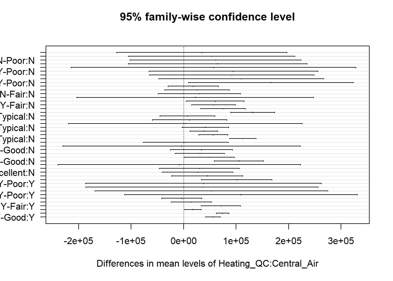
In the giant table above as well as the confidence interval plots, you are able to inspect which combination of categories are statistically different.
With interactions present in ANOVA models, post-hoc tests might get overwhelming in trying to find where differences exist. To help guide the exploration of post-hoc tests with interactions, we can do slicing. Slicing is when you perform One-Way ANOVA on subsets of data within categories of other variables. Even though the interaction in our model was not significant, let’s imagine that it was for the sake of example. For example, to help discover differences in the interaction between central air and heating quality, we could subset the data into two groups - homes with central air and homes without. Within these two groups we perform One-Way ANOVA across heating quality to find where differences might exist within subgroups.
This can easily be done with the group_by function to subset the data. The nest and mutate functions are also used to applied the aov function to each subgroup. Here we run a One-Way ANOVA for heating quality within each subset of central air being present or not.
CA_aov <- train %>%
  group_by(Central_Air) %>%
  nest() %>%
  mutate(aov = map(data, ~summary(aov(Sale_Price ~ Heating_QC, data = .x))))

CA_aov
## # A tibble: 2 × 3
## # Groups: Central_Air [2]
## Central_Air data aov
## <fct> <list> <list>
## 1 Y <tibble [1,904 × 81]> <summry.v>
## 2 N <tibble [147 × 81]> <summry.v>## [[1]]
## Df Sum Sq Mean Sq F value Pr(>F)
## Heating_QC 4 2.242e+12 5.606e+11 108.5 <2e-16 ***
## Residuals 1899 9.809e+12 5.165e+09
## ---
## Signif. codes: 0 '***' 0.001 '**' 0.01 '*' 0.05 '.' 0.1 ' ' 1
##
## [[2]]
## Df Sum Sq Mean Sq F value Pr(>F)
## Heating_QC 4 1.774e+10 4.435e+09 3.793 0.00582 **
## Residuals 142 1.660e+11 1.169e+09
## ---
## Signif. codes: 0 '***' 0.001 '**' 0.01 '*' 0.05 '.' 0.1 ' ' 1We can see that both of these results are significant at the 0.05 level. This implies that there are statistical differences in average sale price across heating quality within homes that have central air as well as those that don’t have central air.
3.2.2 Assumptions
The assumptions for the \(n\)-Way ANOVA are the same as with the One-Way ANOVA - independence of observations, normality for each category of variable, and equal variances. With the inclusion of two or more variables (\(n\)-Way ANOVA with \(n > 1\)), these assumptions can be harder to evaluate and test. These assumptions are then applied to the residuals of the model.
For equal variances, we can still apply the Levene Test for equal variances using the same leveneTest function as in Chapter 2.
## Levene's Test for Homogeneity of Variance (center = median)
##         Df F value    Pr(>F)
## group    9   24.17 < 2.2e-16 ***
##       2041
## ---
## Signif. codes:  0 '***' 0.001 '**' 0.01 '*' 0.05 '.' 0.1 ' ' 1
From this test, we can see that we do not meet our assumption of equal variance.
Let’s explore the normality assumption. Again, we will assume this normality on the random error component, \(\varepsilon_{ijk}\), of the ANOVA model. More details are found for diagnostic testing using the error component in Diagnostic chapter. We can check normality using the same approaches of the QQ-plot or statistical testing as in the section on EDA. Here we will use the plot function on the aov object. Specifically, we want the second plot which is why we have a 2 in the plot function option. We then use the shapiro.test function on the error component. The estimate of the error component is calculated using the residuals function.
##
##  Shapiro-Wilk normality test
##
## data:  ames_res
## W = 0.8838, p-value < 2.2e-16
Neither of the normality or equal variance assumptions appear to be met here. This would be a good scenario to have a non-parametric approach. Unfortunately, the Kruskal-Wallis approach is not applicable to \(n\)-Way ANOVA where \(n > 1\). These approaches would need more non-parametric versions of multiple regression models to account for them.
3.2.3 Python Code
Two-way ANOVA with interactions
import matplotlib.pyplot as plt
import scipy as sp
import pandas as pd
import numpy as np


model = smf.ols("Sale_Price ~ C(Heating_QC)*C(Central_Air)", data = train).fit()
model.summary()| Dep. Variable: | Sale_Price | R-squared: | 0.244 |
|---|---|---|---|
| Model: | OLS | Adj. R-squared: | 0.240 |
| Method: | Least Squares | F-statistic: | 73.08 |
| Date: | Tue, 17 Jun 2025 | Prob (F-statistic): | 3.30e-117 |
| Time: | 13:39:05 | Log-Likelihood: | -25801. |
| No. Observations: | 2051 | AIC: | 5.162e+04 |
| Df Residuals: | 2041 | BIC: | 5.168e+04 |
| Df Model: | 9 | ||
| Covariance Type: | nonrobust |
| coef | std err | t | P>|t| | [0.025 | 0.975] | |
|---|---|---|---|---|---|---|
| Intercept | 1.13e+05 | 1.96e+04 | 5.778 | 0.000 | 7.46e+04 | 1.51e+05 |
| C(Heating_QC)[T.Fair] | -2.711e+04 | 2.35e+04 | -1.152 | 0.249 | -7.33e+04 | 1.9e+04 |
| C(Heating_QC)[T.Good] | -5788.8889 | 2.57e+04 | -0.226 | 0.822 | -5.61e+04 | 4.45e+04 |
| C(Heating_QC)[T.Poor] | -6.293e+04 | 5.35e+04 | -1.175 | 0.240 | -1.68e+05 | 4.21e+04 |
| C(Heating_QC)[T.Typical] | -1.083e+04 | 2.12e+04 | -0.512 | 0.609 | -5.23e+04 | 3.07e+04 |
| C(Central_Air)[T.Y] | 1.058e+05 | 1.97e+04 | 5.380 | 0.000 | 6.73e+04 | 1.44e+05 |
| C(Heating_QC)[T.Fair]:C(Central_Air)[T.Y] | -4.076e+04 | 2.65e+04 | -1.540 | 0.124 | -9.27e+04 | 1.11e+04 |
| C(Heating_QC)[T.Good]:C(Central_Air)[T.Y] | -5.557e+04 | 2.61e+04 | -2.133 | 0.033 | -1.07e+05 | -4469.381 |
| C(Heating_QC)[T.Poor]:C(Central_Air)[T.Y] | -4.888e+04 | 8.86e+04 | -0.552 | 0.581 | -2.23e+05 | 1.25e+05 |
| C(Heating_QC)[T.Typical]:C(Central_Air)[T.Y] | -6.208e+04 | 2.15e+04 | -2.888 | 0.004 | -1.04e+05 | -1.99e+04 |
| Omnibus: | 815.967 | Durbin-Watson: | 2.014 |
|---|---|---|---|
| Prob(Omnibus): | 0.000 | Jarque-Bera (JB): | 4837.979 |
| Skew: | 1.771 | Prob(JB): | 0.00 |
| Kurtosis: | 9.638 | Cond. No. | 91.1 |
Notes:
[1] Standard Errors assume that the covariance matrix of the errors is correctly specified.
##                                     sum_sq      df           F        PR(>F)
## C(Heating_QC)                 2.216871e+12     4.0  111.516329  4.580351e-86
## C(Central_Air)                3.390960e+11     1.0   68.230837  2.582411e-16
## C(Heating_QC):C(Central_Air)  4.353317e+10     4.0    2.189870  6.779864e-02
## Residual 1.014343e+13 2041.0 NaN NaNPost-hoc testing
model_slice1 = smf.ols("Sale_Price ~ C(Heating_QC)", data = train[train["Central_Air"] == 'Y']).fit()
model_slice1.summary()| Dep. Variable: | Sale_Price | R-squared: | 0.184 |
|---|---|---|---|
| Model: | OLS | Adj. R-squared: | 0.182 |
| Method: | Least Squares | F-statistic: | 107.7 |
| Date: | Tue, 17 Jun 2025 | Prob (F-statistic): | 7.88e-83 |
| Time: | 13:39:06 | Log-Likelihood: | -24113. |
| No. Observations: | 1913 | AIC: | 4.824e+04 |
| Df Residuals: | 1908 | BIC: | 4.826e+04 |
| Df Model: | 4 | ||
| Covariance Type: | nonrobust |
| coef | std err | t | P>|t| | [0.025 | 0.975] | |
|---|---|---|---|---|---|---|
| Intercept | 2.188e+05 | 2220.937 | 98.521 | 0.000 | 2.14e+05 | 2.23e+05 |
| C(Heating_QC)[T.Fair] | -6.787e+04 | 1.24e+04 | -5.471 | 0.000 | -9.22e+04 | -4.35e+04 |
| C(Heating_QC)[T.Good] | -6.135e+04 | 4629.434 | -13.253 | 0.000 | -7.04e+04 | -5.23e+04 |
| C(Heating_QC)[T.Poor] | -1.118e+05 | 7.22e+04 | -1.548 | 0.122 | -2.53e+05 | 2.99e+04 |
| C(Heating_QC)[T.Typical] | -7.291e+04 | 3908.610 | -18.654 | 0.000 | -8.06e+04 | -6.52e+04 |
| Omnibus: | 745.622 | Durbin-Watson: | 2.043 |
|---|---|---|---|
| Prob(Omnibus): | 0.000 | Jarque-Bera (JB): | 4152.079 |
| Skew: | 1.749 | Prob(JB): | 0.00 |
| Kurtosis: | 9.313 | Cond. No. | 46.1 |
Notes:
[1] Standard Errors assume that the covariance matrix of the errors is correctly specified.
##                      sum_sq      df           F        PR(>F)
## C(Heating_QC)  2.246168e+12     4.0  107.704754  7.875980e-83
## Residual       9.947769e+12  1908.0         NaN           NaN
model_slice2 = smf.ols("Sale_Price ~ C(Heating_QC)", data = train[train["Central_Air"] == 'N']).fit()
model_slice2.summary()| Dep. Variable: | Sale_Price | R-squared: | 0.068 |
|---|---|---|---|
| Model: | OLS | Adj. R-squared: | 0.040 |
| Method: | Least Squares | F-statistic: | 2.419 |
| Date: | Tue, 17 Jun 2025 | Prob (F-statistic): | 0.0516 |
| Time: | 13:39:06 | Log-Likelihood: | -1649.8 |
| No. Observations: | 138 | AIC: | 3310. |
| Df Residuals: | 133 | BIC: | 3324. |
| Df Model: | 4 | ||
| Covariance Type: | nonrobust |
| coef | std err | t | P>|t| | [0.025 | 0.975] | |
|---|---|---|---|---|---|---|
| Intercept | 1.13e+05 | 1.06e+04 | 10.620 | 0.000 | 9.19e+04 | 1.34e+05 |
| C(Heating_QC)[T.Fair] | -2.711e+04 | 1.28e+04 | -2.118 | 0.036 | -5.24e+04 | -1790.733 |
| C(Heating_QC)[T.Good] | -5788.8889 | 1.4e+04 | -0.415 | 0.679 | -3.34e+04 | 2.18e+04 |
| C(Heating_QC)[T.Poor] | -6.292e+04 | 2.91e+04 | -2.160 | 0.033 | -1.21e+05 | -5300.604 |
| C(Heating_QC)[T.Typical] | -1.083e+04 | 1.15e+04 | -0.941 | 0.348 | -3.36e+04 | 1.19e+04 |
| Omnibus: | 40.204 | Durbin-Watson: | 2.083 |
|---|---|---|---|
| Prob(Omnibus): | 0.000 | Jarque-Bera (JB): | 94.171 |
| Skew: | 1.190 | Prob(JB): | 3.56e-21 |
| Kurtosis: | 6.274 | Cond. No. | 11.2 |
Notes:
[1] Standard Errors assume that the covariance matrix of the errors is correctly specified.
##                      sum_sq     df         F    PR(>F)
## C(Heating_QC)  1.423639e+10    4.0  2.419249  0.051615
## Residual       1.956640e+11  133.0       NaN       NaN
Assumptions
## ShapiroResult(statistic=0.8877905358408816, pvalue=3.2424049575361566e-36)3.3 Randomized Block Design
There are two typical groups of data analysis studies that are conducted. The first are observational/retrospective studies which are the typical data problems people try to solve. The primary characteristic of these analysis are looking at what already happened (retrospective) and potentially inferring those results to further data. These studies have little control over other factors contributing to the target of interest because data is collected after the fact.
The other type of data analysis study are controlled experiments. In these situations, you often want to look at the outcome measure prospectively. The focus of the controlled experiment is to control for other factors that might contribute to the target variable. By manipulating these factors of interest, one can more reasonably claim causation. We can more reasonably claim causation when random assignment is used to eliminate potential nuisance factors. Nuisance factors are variables that can potentially impact the target variable, but are not of interest in the analysis directly.
3.3.1 Garlic Bulb Weight Example
For this analysis we will use a new dataset. This dataset contains the average garlic bulb weight from different plots of land. We want to compare the effects of fertilizer on average bulb weight. However, different plots of land could have different levels of sun exposure, pH for the soil, and rain amounts. Since we cannot alter the pH of the soil easily, or control the sun and rain, we can use blocking to account for these nuisance factors. Each fertilizer was randomly applied in quadrants of 8 plots of land. These 8 plots have different values for sun exposure, pH, and rain amount. Therefore, if we only put one fertilizer on each plot, we would not know if the fertilizer was the reason the garlic crop grew or if it was one of the nuisance factors. Since we blocked these 8 plots and applied all four fertilizers in each we have essentially accounted for (or removed the effect of) the nuisance factors.
Let’s briefly explore this new dataset by looking at all 32 values using the print function.
3.3.1.1 R code:
## Rows: 32 Columns: 6
## ── Column specification ────────────────────────────────────────────────────────
## Delimiter: ","
## dbl (6): Sector, Position, Fertilizer, BulbWt, Cloves, BedId
##
## ℹ Use `spec()` to retrieve the full column specification for this data.
## ℹ Specify the column types or set `show_col_types = FALSE` to quiet this message.## # A tibble: 32 × 6
## Sector Position Fertilizer BulbWt Cloves BedId
## <dbl> <dbl> <dbl> <dbl> <dbl> <dbl>
## 1 1 1 3 0.259 11.6 22961
## 2 1 2 4 0.207 12.6 23884
## 3 1 3 1 0.275 12.1 19642
## 4 1 4 2 0.245 12.1 20384
## 5 2 1 3 0.215 11.6 20303
## 6 2 2 4 0.170 12.7 21004
## 7 2 3 1 0.225 12.0 16117
## 8 2 4 2 0.168 11.9 19686
## 9 3 1 4 0.217 12.4 26527
## 10 3 2 3 0.226 11.7 23574
## # ℹ 22 more rowsHow do we account for this blocking in an ANOVA model context? This blocking ANOVA model is the exact same as the Two-Way ANOVA model. The variable that identifies which sector (block) an observation is in serves as another variable in the model. Think about this variable as the variable that accounts for all the nuisance factors in your ANOVA. That means we have two variables in this ANOVA model - fertilizer and sector (the block that accounts for sun exposure, pH level of soil, rain amount, etc.).
For this we can use the same aov function we described above.
##                    Df   Sum Sq   Mean Sq F value   Pr(>F)
## factor(Fertilizer)  3 0.005086 0.0016954   4.307 0.016222 *
## factor(Sector)      7 0.017986 0.0025695   6.527 0.000364 ***
## Residuals          21 0.008267 0.0003937
## ---
## Signif. codes:  0 '***' 0.001 '**' 0.01 '*' 0.05 '.' 0.1 ' ' 1
Using the summary function we can see that both the sector (block) and fertilizer variables are significant in the model at the 0.05 level. What are the interpretations of this?
First, let’s address the blocking variable. Whether it is significant or not, it should always be included in the model. This is due to the fact that the data is structured in that way. It is a construct of the data that should be accounted for regardless of the significance. However, since the blocking variable (sector) was significant, that implies that different plots of land have different impacts of the average bulb weight of garlic. Again, this is most likely due to the differences between the plots of land - namely sun exposure, pH of soil, rain fall, etc.
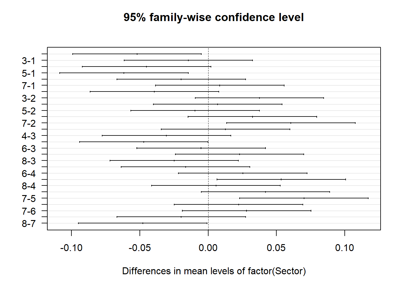
Second, the variable of interest is the fertilizer variable. It is significant, implying that there is a difference in the average bulb weight of garlic for different fertilizers. To examine which fertilizer pairs are statistically difference we can use post-hos testing as described in the previous parts of this chapter using the TukeyHSD function.
##   Tukey multiple comparisons of means
##     95% family-wise confidence level
##
## Fit: aov(formula = BulbWt ~ factor(Fertilizer) + factor(Sector), data = block)
##
## $`factor(Fertilizer)`
##            diff         lwr          upr     p adj
## 2-1 -0.02509875 -0.05275125  0.002553751 0.0840024
## 3-1 -0.01294875 -0.04060125  0.014703751 0.5698678
## 4-1 -0.03336125 -0.06101375 -0.005708749 0.0144260
## 3-2  0.01215000 -0.01550250  0.039802501 0.6186232
## 4-2 -0.00826250 -0.03591500  0.019390001 0.8382800
## 4-3 -0.02041250 -0.04806500  0.007240001 0.1995492
##
## $`factor(Sector)`
##           diff          lwr           upr     p adj
## 2-1 -0.0520675 -0.099126544 -5.008456e-03 0.0234315
## 3-1 -0.0145075 -0.061566544  3.255154e-02 0.9634255
## 4-1 -0.0450550 -0.092114044  2.004044e-03 0.0669646
## 5-1 -0.0616250 -0.108684044 -1.456596e-02 0.0051483
## 6-1 -0.0196650 -0.066724044  2.739404e-02 0.8466335
## 7-1  0.0084950 -0.038564044  5.555404e-02 0.9984089
## 8-1 -0.0393325 -0.086391544  7.726544e-03 0.1469768
## 3-2  0.0375600 -0.009499044  8.461904e-02 0.1841786
## 4-2  0.0070125 -0.040046544  5.407154e-02 0.9995370
## 5-2 -0.0095575 -0.056616544  3.750154e-02 0.9966777
## 6-2  0.0324025 -0.014656544  7.946154e-02 0.3337758
## 7-2  0.0605625  0.013503456  1.076215e-01 0.0061094
## 8-2  0.0127350 -0.034324044  5.979404e-02 0.9819446
## 4-3 -0.0305475 -0.077606544  1.651154e-02 0.4025951
## 5-3 -0.0471175 -0.094176544 -5.845586e-05 0.0495704
## 6-3 -0.0051575 -0.052216544  4.190154e-02 0.9999400
## 7-3  0.0230025 -0.024056544  7.006154e-02 0.7227812
## 8-3 -0.0248250 -0.071884044  2.223404e-02 0.6454690
## 5-4 -0.0165700 -0.063629044  3.048904e-02 0.9286987
## 6-4  0.0253900 -0.021669044  7.244904e-02 0.6208608
## 7-4  0.0535500  0.006490956  1.006090e-01 0.0186102
## 8-4  0.0057225 -0.041336544  5.278154e-02 0.9998793
## 6-5  0.0419600 -0.005099044  8.901904e-02 0.1034664
## 7-5  0.0701200  0.023060956  1.171790e-01 0.0012997
## 8-5  0.0222925 -0.024766544  6.935154e-02 0.7514897
## 7-6  0.0281600 -0.018899044  7.521904e-02 0.5004099
## 8-6 -0.0196675 -0.066726544  2.739154e-02 0.8465530
## 8-7 -0.0478275 -0.094886544 -7.684559e-04 0.0446174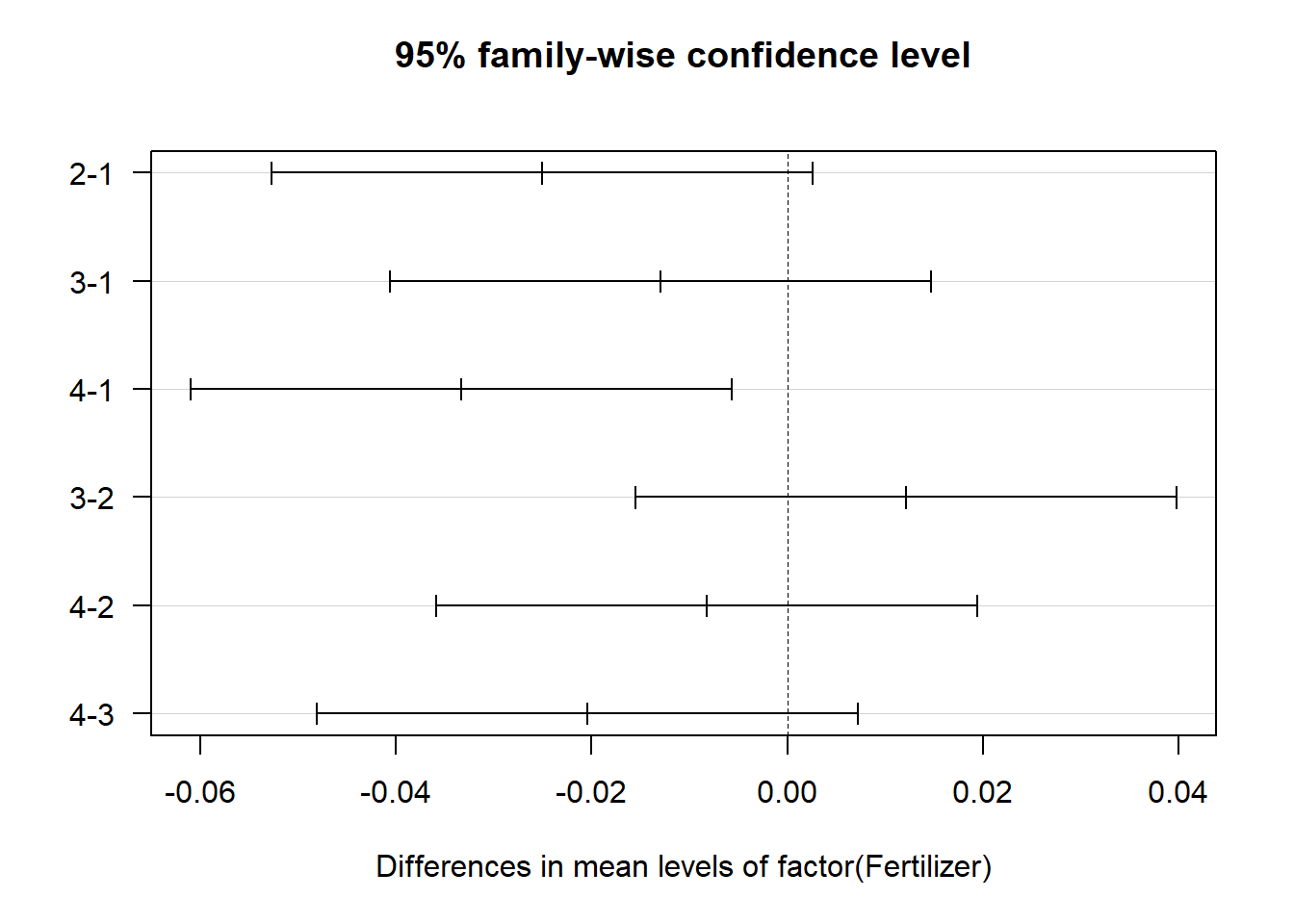
3.3.2 Assumptions
Outside of the typical assumptions for ANOVA that still hold here, there are two additional assumptions to be met:
- Treatments are randomly assigned within each block
- The effects of the treatment variable are constant across the levels of the blocking variable
The first, new assumption of randomness deals with the reliability of the analysis. Randomness is key to removing the impact of the nuisance factors. The second, new assumption implies there is no interaction between the treatment variable and the blocking variable. For example, we are implying that the fertilizers’ impacts ob garlic bulb weight are not changed depending on what block you are on. In other words, fertilizers have the same impact regardless of sun exposure, pH levels, rain fall, etc. We are not saying these nuisance factors do not impact the target variable or bulb weight of garlic, just that they do not change the effect of the fertilizer on bulb weight.
3.3.3 Python Code
block=pd.read_csv('https://raw.githubusercontent.com/IAA-Faculty/statistical_foundations/master/garlic_block.csv')
block.head(n = 32)
## Sector Position Fertilizer BulbWt Cloves BedId
## 0 1 1 3 0.25881 11.6322 22961
## 1 1 2 4 0.20746 12.5837 23884
## 2 1 3 1 0.27453 12.0597 19642
## 3 1 4 2 0.24467 12.1001 20384
## 4 2 1 3 0.21454 11.5863 20303
## 5 2 2 4 0.16953 12.7132 21004
## 6 2 3 1 0.22504 12.0470 16117
## 7 2 4 2 0.16809 11.9071 19686
## 8 3 1 4 0.21720 12.3655 26527
## 9 3 2 3 0.22551 11.6864 23574
## 10 3 3 2 0.23536 12.0258 17499
## 11 3 4 1 0.24937 11.6668 16636
## 12 4 1 4 0.20811 12.5996 24834
## 13 4 2 1 0.21138 12.1393 19946
## 14 4 3 2 0.19320 12.0792 21504
## 15 4 4 3 0.19256 11.6464 23181
## 16 5 1 4 0.19851 12.5355 24533
## 17 5 2 1 0.18603 12.3307 15009
## 18 5 3 3 0.19698 11.5608 23845
## 19 5 4 2 0.15745 11.8735 18948
## 20 6 1 2 0.20058 11.9077 20019
## 21 6 2 3 0.25346 11.7294 22228
## 22 6 3 4 0.19838 12.7670 24424
## 23 6 4 1 0.25439 12.0139 13755
## 24 7 1 3 0.26578 11.7448 21087
## 25 7 2 4 0.21678 12.8531 25751
## 26 7 3 2 0.26183 12.3990 20296
## 27 7 4 1 0.27506 11.9383 20038
## 28 8 1 1 0.21420 12.1034 17843
## 29 8 2 3 0.17877 11.5682 21394
## 30 8 3 4 0.20714 12.5213 27191
## 31 8 4 2 0.22803 12.2317 20202import statsmodels.formula.api as smf
model_b = smf.ols("BulbWt ~ C(Fertilizer) + C(Sector)", data = block).fit()
model_b.summary()| Dep. Variable: | BulbWt | R-squared: | 0.736 |
|---|---|---|---|
| Model: | OLS | Adj. R-squared: | 0.611 |
| Method: | Least Squares | F-statistic: | 5.861 |
| Date: | Tue, 17 Jun 2025 | Prob (F-statistic): | 0.000328 |
| Time: | 13:39:07 | Log-Likelihood: | 86.773 |
| No. Observations: | 32 | AIC: | -151.5 |
| Df Residuals: | 21 | BIC: | -135.4 |
| Df Model: | 10 | ||
| Covariance Type: | nonrobust |
| coef | std err | t | P>|t| | [0.025 | 0.975] | |
|---|---|---|---|---|---|---|
| Intercept | 0.2642 | 0.012 | 22.713 | 0.000 | 0.240 | 0.288 |
| C(Fertilizer)[T.2] | -0.0251 | 0.010 | -2.530 | 0.019 | -0.046 | -0.004 |
| C(Fertilizer)[T.3] | -0.0129 | 0.010 | -1.305 | 0.206 | -0.034 | 0.008 |
| C(Fertilizer)[T.4] | -0.0334 | 0.010 | -3.363 | 0.003 | -0.054 | -0.013 |
| C(Sector)[T.2] | -0.0521 | 0.014 | -3.711 | 0.001 | -0.081 | -0.023 |
| C(Sector)[T.3] | -0.0145 | 0.014 | -1.034 | 0.313 | -0.044 | 0.015 |
| C(Sector)[T.4] | -0.0451 | 0.014 | -3.211 | 0.004 | -0.074 | -0.016 |
| C(Sector)[T.5] | -0.0616 | 0.014 | -4.392 | 0.000 | -0.091 | -0.032 |
| C(Sector)[T.6] | -0.0197 | 0.014 | -1.402 | 0.176 | -0.049 | 0.010 |
| C(Sector)[T.7] | 0.0085 | 0.014 | 0.605 | 0.551 | -0.021 | 0.038 |
| C(Sector)[T.8] | -0.0393 | 0.014 | -2.803 | 0.011 | -0.069 | -0.010 |
| Omnibus: | 1.984 | Durbin-Watson: | 2.574 |
|---|---|---|---|
| Prob(Omnibus): | 0.371 | Jarque-Bera (JB): | 1.162 |
| Skew: | -0.071 | Prob(JB): | 0.559 |
| Kurtosis: | 2.077 | Cond. No. | 9.67 |
Notes:
[1] Standard Errors assume that the covariance matrix of the errors is correctly specified.
##                  sum_sq    df         F    PR(>F)
## C(Fertilizer)  0.005086   3.0  4.306540  0.016222
## C(Sector)      0.017986   7.0  6.526673  0.000364
## Residual       0.008267  21.0       NaN       NaN
3.4 Multiple Linear Regression
Most practical applications of of regression modeling involve using more complicated models than a simple linear regression with only one predictor variable to predict your target. Additional variables in a model can lead to better explanations and predictions of the target. These linear regressions with more than one variable are called multiple linear regression models. However, as we will see in this section and the following chapters, with more variables comes much more complication.
3.4.1 Model Structure
Multiple linear regression models have the same structure as simple linear regression models, only with more variables. The multiple linear regression model with \(k\) variables is structured like the following:
\[ y = \beta_0 + \beta_1 x_1 + \beta_2 x_2 + \cdots + \beta_k x_k + \varepsilon \]
This model has the predictor variables \(x_1, x_2, ..., x_k\) trying to either explain or predict the target variable \(y\). The intercept, \(\beta_0\), still gives the expected value of \(y\), when all of the predictor variables take a value of 0. With the addition of multiple predictors, the interpretation of the slope coefficients change slightly. The slopes, \(\beta_1, \beta_2, ..., \beta_k\), give the expected change in \(y\) for a one unit change in the respective predictor variable, holding all other predictor variables constant. The random error term, \(\varepsilon\), is the error between our predicted value, \(\hat{y} = \hat{\beta}_0 + \hat{\beta}_1 x_1 + \cdots + \hat{\beta}_k x_k\), and our actual value of \(y\).
Unlike simple linear regression that can be visualized as a line through a 2-dimensional scatterplot of data, a multiple linear regression is better thought of as a multi-dimensional plane through a multi-dimensional scatterplot of data.
Let’s visual an example with two predictor variables - the square footage of greater living area and the total number of rooms. These will predict sale price of a home. When none of the variables have any relationship with the target variable, we get a horizontal plane like the one shown below. This is similar in concept to a horizontal line in simple linear regression having a slope of 0, implying that the target variable does not change as the predictor variable changes.
3.4.1.1 R code:
Much like if the slope of a simple linear regression line is not 0 (a relationship exists between the predictor and target variable), then a relationship between any of the predictor variables and the target variable shifts and rotates the plane around like the one shown below.
To the naive viewer, the shifted plane would still make sense because of the model naming convention of multiple linear regression. However, the linear in linear regression doesn’t have to deal with the visualization of the fitted plane (or line in two dimensions), but instead refers to the linear combination of variables. A linear combination is an expression constructed from a set of terms by multiplying each term by a constant and adding the results. For example, \(ax + by\) is a linear combination of \(x\) and \(y\). Therefore, the linear model
\[ y = \beta_0 + \beta_1 x_1 + \beta_2 x_2 + \cdots + \beta_k x_k + \varepsilon \] is a linear combination of predictor variables in their relationship with the target variable \(y\). These predictor variables do not all have to contain linear effects though. For example, let’s look at a linear regression model with four predictor variables:
\[ y = \beta_0 + \beta_1 x_1 + \beta_2 x_2 + \beta_3 x_3 + \beta_4 x_4 + \varepsilon \]
One would not be hard pressed to call this model a linear regression. However, what if we defined \(x_3 = x_1^2\) and \(x_4 = x_2^2\)?
This model is still a linear regression model. The structure of the model did not change. The model is still a linear combination of predictor variables related to the target variable. The predictor variables just do not all have a linear effect in terms of their relationship with \(y\). However, mathematically, it is still a linear combination and a linear regression model.
3.4.2 Global & Local Inference
In simple linear regression we could just look at the t-test for our slope parameter estimate to determine the utility of our model. With multiple parameter estimates comes multiple t-tests. Instead of looking at every individual parameter estimate initially, there is a way to determine the model adequacy for predicting the target variable overall.
The utility of a multiple regression model can be tested with a single test that encompasses all the coefficients from the model. This kind of test is called a global test since it tests all \(\beta\)’s simultaneously. The Global F-Test uses the F-distribution to do just that for multiple linear regression models. The hypotheses for this test are the following:
\[ H_0: \beta_1 = \beta_2 = \cdots = \beta_k = 0 \\ H_A: \text{at least one } \beta \text{ is nonzero} \]
In simpler terms, the null hypothesis is that none of the variables are useful in predicting the target variable. The alternative hypothesis is that at least one of these variables is useful in predicting the target variable.
The F-distribution is a distribution that has the following characteristics:
- Bounded below by 0
- Right-skewed
- Both numerator and denominator degrees of freedom
A plot of a variety of F distributions is shown here:
## Warning: Removed 1500 rows containing missing values or values outside the scale range
## (`geom_line()`).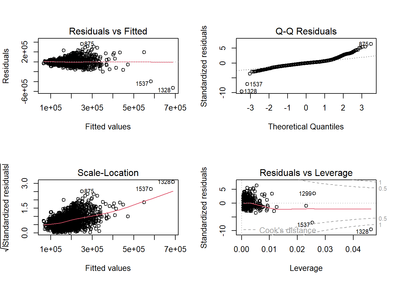
If the global test is significant, the next step would be to examine the individual t-tests to see which variables are significant and which ones are not. This is similar to post-hoc testing in ANOVA where we explored which of the categories was statistically different when we knew at least one was.
These tests are all available using the summary function on an lm function for linear regression. To build a multiple linear regression in R using the lm function, you just add another variable to the formula element. Here we will predict the sales price (Sale_Price) based on the square footage of the greater living area of the home (Gr_Liv_Area) as well as total number of rooms above ground (TotRms_AbvGrd).
##
## Call:
## lm(formula = Sale_Price ~ Gr_Liv_Area + TotRms_AbvGrd, data = train)
##
## Residuals:
##     Min      1Q  Median      3Q     Max
## -528656  -30077   -1230   21427  361465
##
## Coefficients:
##                 Estimate Std. Error t value Pr(>|t|)
## (Intercept)    42562.657   5365.721   7.932 3.51e-15 ***
## Gr_Liv_Area      136.982      4.207  32.558  < 2e-16 ***
## TotRms_AbvGrd -10563.324   1370.007  -7.710 1.94e-14 ***
## ---
## Signif. codes:  0 '***' 0.001 '**' 0.01 '*' 0.05 '.' 0.1 ' ' 1
##
## Residual standard error: 56630 on 2048 degrees of freedom
## Multiple R-squared:  0.5024, Adjusted R-squared:  0.5019
## F-statistic:  1034 on 2 and 2048 DF,  p-value: < 2.2e-16
At the bottom of the above output is the result of the global F-test. Since the p-value on this test is lower than the significance level of 0.05, we have statistical evidence that at least of the two variables - Gr_Liv_Area and TotRms_AbvGrd - is significant at predicting the sale price of the home. By looking at the individual t-tests in the output above, we can see that both variables are actually significant.
3.4.3 Assumptions
The main assumptions for the multiple linear regression model are the same as with the simple linear regression model:
- The expected value of \(y\) is linear in the \(x\)’s (proper model specification).
- The random errors are independent.
- The random errors are normally distributed.
- The random errors have equal variance (homoskedasticity).
However, with multiple variables there is an additional assumption that people tend to add to multiple linear regression modeling:
- No perfect collinearity (also called multicollinearity)
The new assumption means that no combination of predictor variables is a perfect linear combination with any other predictor variables. Collinearity, also called multicollinearity, occurs when predictor variables are correlated with each other. People often misstate this additional assumption as having no collinearity at all. This is too restrictive and basically impossible to meet in a realistic setting. Only when collinearity has a drastic impact on the linear regression do we need to concern ourselves. In fact, linear regression only completely breaks when that collinearity is perfect. Dealing with multicollinearity is discussed later.
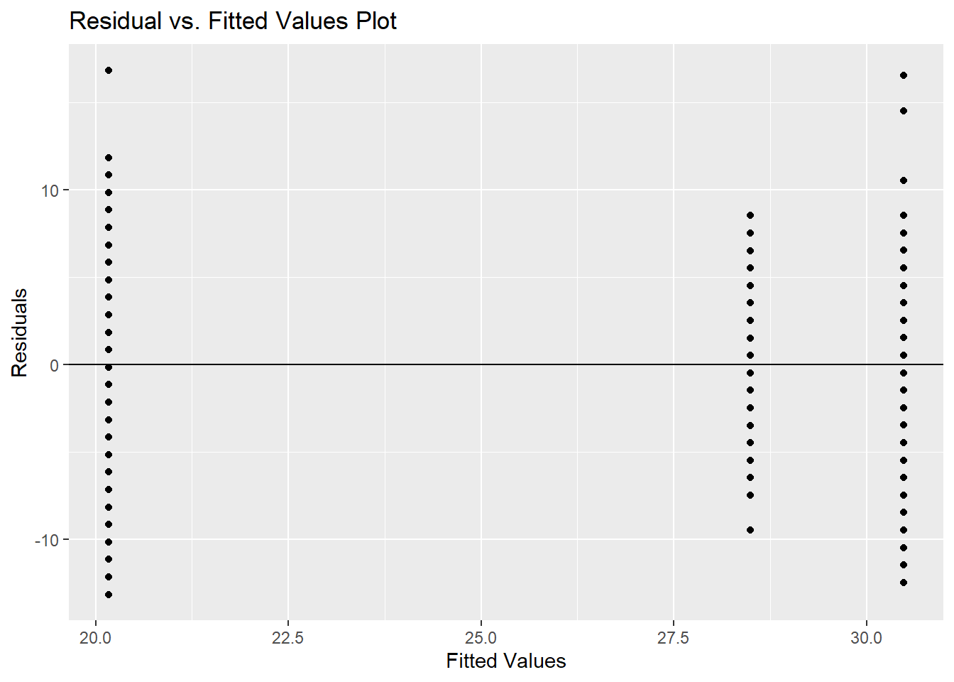
Similar to simple linear regression, we can evaluate the assumptions by looking at residual plots. The plot function on the lm object provides these.

These will again be covered in much more detail in Diagnostic Chapter.
3.4.4 Multiple Coefficients of Determination
One of the main advantages of multiple linear regression is that the complexity of the model enables us to investigate the relationship among \(y\) and several predictor variables simultaneously. However, this increased complexity makes it more difficult to not only interpret the models, but also ascertain which model is “best.”
One example of this would be the coefficient of determination, \(R^2\), that we discussed earlier. The calculation for \(R^2\) is the exact same:
\[ R^2 = 1 - \frac{SSE}{TSS} \]
However, the problem with the calculation of \(R^2\) in a multiple linear regression is that the addition of any variable (useful or not) will never make the \(R^2\) decrease. In fact, it typically increases even with the addition of a useless variable. The reason is rather intuitive. When adding information to a regression model, your predictions can only get better, not worse. If a new predictor variable has no impact on the target variable, then the predictions can not get any worse than what they already were before the addition of the useless variable. Therefore, the \(SSE\) would never increase, making the \(R^2\) never decrease.
To account for this problem, there is the adjusted coefficient of determination, \(R^2_a\). The calculation is the following:
\[ R^2_a = 1 - [(\frac{n-1}{n-(k+1)})\times (\frac{SSE}{TSS})] \]
Notice what the calculation is doing. It takes the original ratio on the right hand side of the \(R^2\) equation, \(SSE/TSS\), and penalizes it. It multiplies this number by a ratio that is always greater than 1 if \(k > 0\). Remember, \(k\) is the number of variables in the model. Therefore, as the number of variables increases, the calculation penalizes the model more and more. However, if the reduction of SSE from adding a useful variable is low enough, then even with the additional penalization, the \(R^2_a\) will increase if the variable is a useful addition to the model. If the variable is not a useful addition to the model, the \(R^2_a\) will decrease. The \(R^2_a\) is only one of many ways to select the “best” model for multiple linear regression.
One downside of this new metric is that the \(R^2_a\) loses its interpretation. Since \(R^2_a \le R^2\), it is no longer bounded below by zero. Therefore, it can no longer be the proportion of variation explained in the target variable by the model. However, we can easily use \(R^2_a\) to select a model correctly and interpret that model with \(R^2\). Both of these numbers can be found using the summary function on the lm object from the previous model.
##
## Call:
## lm(formula = Sale_Price ~ Gr_Liv_Area + TotRms_AbvGrd, data = train)
##
## Residuals:
##     Min      1Q  Median      3Q     Max
## -528656  -30077   -1230   21427  361465
##
## Coefficients:
##                 Estimate Std. Error t value Pr(>|t|)
## (Intercept)    42562.657   5365.721   7.932 3.51e-15 ***
## Gr_Liv_Area      136.982      4.207  32.558  < 2e-16 ***
## TotRms_AbvGrd -10563.324   1370.007  -7.710 1.94e-14 ***
## ---
## Signif. codes:  0 '***' 0.001 '**' 0.01 '*' 0.05 '.' 0.1 ' ' 1
##
## Residual standard error: 56630 on 2048 degrees of freedom
## Multiple R-squared:  0.5024, Adjusted R-squared:  0.5019
## F-statistic:  1034 on 2 and 2048 DF,  p-value: < 2.2e-16
From this output we can say that the combination of Gr_Liv_Area and TotRmsAbvGrd account for 50.24% of the variation in Sale_Price. Now let’s add a random variable to the model. This random variable will take random values from a normal distribution with mean of 0 and standard deviation of 1 and has no impact on the target variable.
set.seed(1234)
ames_lm3 <- lm(Sale_Price ~ Gr_Liv_Area + TotRms_AbvGrd + rnorm(length(Sale_Price), 0, 1), data = train)

summary(ames_lm3)
##
## Call:
## lm(formula = Sale_Price ~ Gr_Liv_Area + TotRms_AbvGrd + rnorm(length(Sale_Price),
## 0, 1), data = train)
##
## Residuals:
## Min 1Q Median 3Q Max
## -527926 -29943 -1298 21427 363925
##
## Coefficients:
## Estimate Std. Error t value Pr(>|t|)
## (Intercept) 42589.091 5364.877 7.939 3.34e-15 ***
## Gr_Liv_Area 136.927 4.207 32.548 < 2e-16 ***
## TotRms_AbvGrd -10552.425 1369.808 -7.704 2.05e-14 ***
## rnorm(length(Sale_Price), 0, 1) 1629.854 1259.478 1.294 0.196
## ---
## Signif. codes: 0 '***' 0.001 '**' 0.01 '*' 0.05 '.' 0.1 ' ' 1
##
## Residual standard error: 56620 on 2047 degrees of freedom
## Multiple R-squared: 0.5028, Adjusted R-squared: 0.502
## F-statistic: 689.9 on 3 and 2047 DF, p-value: < 2.2e-16Notice that the \(R^2\) of this model actually increased to 0.5028 from 0.5024. However, the \(R^2_a\) value stayed approximately the same at 0.502 since the addition of this new variable did not provide enough predictive power to outweigh the penalty of adding it.
3.4.5 Categorical Predictor Variables
As mentioned in EDA Section, there are two types of variables typically used in modeling:
- Quantitative (or numeric)
- Qualitative (or categorical)
Categorical variables need to be coded differently because they are not numerical in nature. As mentioned in EDA Section, two common coding techniques for linear regression are reference and effects coding. The interpretation of the coefficients (\(\beta\)’s) of these variables in a regression model depend on the specific coding used. The predictions from the model, however, will remain the same regardless of the specific coding that is used.
Let’s use the example of the Central_Air variable with 2 categories - Y and N. Using reference coding, the reference coded variable to describe these 2 categories (with N as the reference level) would be the following:
| Central Air | X1 |
| Y | 1 |
| N | 0 |
The linear regression equation would be:
\[ \hat{y} = \hat{\beta}_0 + \hat{\beta}_1 X_1 \]
Let’s see the mathematical interpretation of the coefficient \(\hat{\beta}_1\). To do this, let’s get the average sale price of a home prediction for a home with central air (\(\hat{y}_Y\)) and without central air (\(\hat{y}_N\)):
\[ \hat{y}_Y = \hat{\beta}_0 + \hat{\beta}_1 \cdot 1 = \hat{\beta}_0 + \hat{\beta}_1 \\ \hat{y}_N = \hat{\beta}_0 + \hat{\beta}_1 \cdot 0 = \hat{\beta}_0 \]
By subtracting these two equations (\(\hat{y}_Y - \hat{y}_N = \hat{\beta}_1\)), we can get the prediction for the average difference in price between a home with central air and without central air. This shows that in reference coding, the coefficient on each dummy variable is the average difference between that category and the reference category (the category not represented with its own variable). The math can be extended to as many categories as needed.
Using effects coding, the effects coded variable to describe these 2 categories (with N as the reference level) would be the following:
| Central Air | X1 |
| Y | 1 |
| N | -1 |
The linear regression equation would be:
\[ \hat{y} = \hat{\beta}_0 + \hat{\beta}_1 X_1 \]
Let’s see the mathematical interpretation of the coefficient \(\hat{\beta}_1\). To do this, let’s get the average sale price of a home prediction for a home with central air (\(\hat{y}_Y\)) and without central air (\(\hat{y}_N\)):
\[ \hat{y}_Y = \hat{\beta}_0 + \hat{\beta}_1 \cdot 1 = \hat{\beta}_0 + \hat{\beta}_1 \\ \hat{y}_N = \hat{\beta}_0 + \hat{\beta}_1 \cdot -1 = \hat{\beta}_0 - \hat{\beta}_1 \]
Similar to reference coding, the coefficient \(\hat{\beta}_1\) is the average difference between homes with central air and \(\hat{\beta}_0\). However, what is \(\hat{\beta}_0\)? By taking the average of our two predictions:
\[ \frac{1}{2} \times (\hat{y}_Y + \hat{y}_N) = \frac{1}{2} \times (\hat{\beta}_0 + \hat{\beta}_1 + \hat{\beta}_0 - \hat{\beta}_1) = \frac{1}{2} \times (2\hat{\beta}_0) = \hat{\beta}_0 \]
From this average we can get the prediction for the average difference in price between a home with central air and the average price across all homes. This shows that in effects coding, the coefficient on each dummy variable is the average difference between that category and the average price across all homes (including both with and without central air). The math can be extended to as many categories as needed.
Let’s see an example with Central_Air as a variable added to our multiple linear regression model as a reference coded variable.
ames_lm4 <- lm(Sale_Price ~ Gr_Liv_Area + TotRms_AbvGrd + Central_Air, data = train)

summary(ames_lm4)
##
## Call:
## lm(formula = Sale_Price ~ Gr_Liv_Area + TotRms_AbvGrd + Central_Air,
## data = train)
##
## Residuals:
## Min 1Q Median 3Q Max
## -510745 -28984 -2317 20273 356742
##
## Coefficients:
## Estimate Std. Error t value Pr(>|t|)
## (Intercept) -7169.259 6778.879 -1.058 0.29
## Gr_Liv_Area 129.594 4.131 31.374 < 2e-16 ***
## TotRms_AbvGrd -8980.938 1335.669 -6.724 2.29e-11 ***
## Central_AirY 54513.082 4762.926 11.445 < 2e-16 ***
## ---
## Signif. codes: 0 '***' 0.001 '**' 0.01 '*' 0.05 '.' 0.1 ' ' 1
##
## Residual standard error: 54910 on 2047 degrees of freedom
## Multiple R-squared: 0.5323, Adjusted R-squared: 0.5316
## F-statistic: 776.6 on 3 and 2047 DF, p-value: < 2.2e-16With these results we estimate the average difference in sales price between homes with central air and without central air to be $54,513.08.
3.4.6 Python Code
Global and Local Inference
model_mlr = smf.ols("Sale_Price ~ Gr_Liv_Area + TotRms_AbvGrd", data = train).fit()
model_mlr.summary()| Dep. Variable: | Sale_Price | R-squared: | 0.499 |
|---|---|---|---|
| Model: | OLS | Adj. R-squared: | 0.499 |
| Method: | Least Squares | F-statistic: | 1022. |
| Date: | Tue, 17 Jun 2025 | Prob (F-statistic): | 1.82e-308 |
| Time: | 13:39:09 | Log-Likelihood: | -25378. |
| No. Observations: | 2051 | AIC: | 5.076e+04 |
| Df Residuals: | 2048 | BIC: | 5.078e+04 |
| Df Model: | 2 | ||
| Covariance Type: | nonrobust |
| coef | std err | t | P>|t| | [0.025 | 0.975] | |
|---|---|---|---|---|---|---|
| Intercept | 4.435e+04 | 5356.883 | 8.279 | 0.000 | 3.38e+04 | 5.49e+04 |
| Gr_Liv_Area | 137.0996 | 4.182 | 32.783 | 0.000 | 128.898 | 145.301 |
| TotRms_AbvGrd | -1.061e+04 | 1344.500 | -7.892 | 0.000 | -1.32e+04 | -7974.412 |
| Omnibus: | 369.235 | Durbin-Watson: | 2.044 |
|---|---|---|---|
| Prob(Omnibus): | 0.000 | Jarque-Bera (JB): | 6501.598 |
| Skew: | 0.299 | Prob(JB): | 0.00 |
| Kurtosis: | 11.702 | Cond. No. | 6.83e+03 |
Notes:
[1] Standard Errors assume that the covariance matrix of the errors is correctly specified.
[2] The condition number is large, 6.83e+03. This might indicate that there are
strong multicollinearity or other numerical problems.
Assumptions
train['pred_mlr'] = model_mlr.predict()
train['resid_mlr'] = model_mlr.resid

p = (
    ggplot(train, aes(sample="resid_mlr")) +
    geom_qq() +
    geom_qq_line(color="blue", linetype="dashed") +
    labs(title="QQ Plot of Residuals", x="Theoretical Quantiles", y="Sample Quantiles")
)

p.show()
Multiple Coefficient of Determination
| Dep. Variable: | Sale_Price | R-squared: | 0.499 |
|---|---|---|---|
| Model: | OLS | Adj. R-squared: | 0.499 |
| Method: | Least Squares | F-statistic: | 1022. |
| Date: | Tue, 17 Jun 2025 | Prob (F-statistic): | 1.82e-308 |
| Time: | 13:39:09 | Log-Likelihood: | -25378. |
| No. Observations: | 2051 | AIC: | 5.076e+04 |
| Df Residuals: | 2048 | BIC: | 5.078e+04 |
| Df Model: | 2 | ||
| Covariance Type: | nonrobust |
| coef | std err | t | P>|t| | [0.025 | 0.975] | |
|---|---|---|---|---|---|---|
| Intercept | 4.435e+04 | 5356.883 | 8.279 | 0.000 | 3.38e+04 | 5.49e+04 |
| Gr_Liv_Area | 137.0996 | 4.182 | 32.783 | 0.000 | 128.898 | 145.301 |
| TotRms_AbvGrd | -1.061e+04 | 1344.500 | -7.892 | 0.000 | -1.32e+04 | -7974.412 |
| Omnibus: | 369.235 | Durbin-Watson: | 2.044 |
|---|---|---|---|
| Prob(Omnibus): | 0.000 | Jarque-Bera (JB): | 6501.598 |
| Skew: | 0.299 | Prob(JB): | 0.00 |
| Kurtosis: | 11.702 | Cond. No. | 6.83e+03 |
Notes:
[1] Standard Errors assume that the covariance matrix of the errors is correctly specified.
[2] The condition number is large, 6.83e+03. This might indicate that there are
strong multicollinearity or other numerical problems.
Categorical Predictor Variables
model_mlr2 = smf.ols("Sale_Price ~ Gr_Liv_Area + TotRms_AbvGrd + C(Central_Air)", data = train).fit()
model_mlr2.summary()| Dep. Variable: | Sale_Price | R-squared: | 0.527 |
|---|---|---|---|
| Model: | OLS | Adj. R-squared: | 0.527 |
| Method: | Least Squares | F-statistic: | 761.8 |
| Date: | Tue, 17 Jun 2025 | Prob (F-statistic): | 0.00 |
| Time: | 13:39:09 | Log-Likelihood: | -25319. |
| No. Observations: | 2051 | AIC: | 5.065e+04 |
| Df Residuals: | 2047 | BIC: | 5.067e+04 |
| Df Model: | 3 | ||
| Covariance Type: | nonrobust |
| coef | std err | t | P>|t| | [0.025 | 0.975] | |
|---|---|---|---|---|---|---|
| Intercept | -6090.0603 | 6929.420 | -0.879 | 0.380 | -1.97e+04 | 7499.388 |
| C(Central_Air)[T.Y] | 5.5e+04 | 4986.530 | 11.029 | 0.000 | 4.52e+04 | 6.48e+04 |
| Gr_Liv_Area | 129.0535 | 4.129 | 31.255 | 0.000 | 120.956 | 137.151 |
| TotRms_AbvGrd | -8868.5091 | 1316.089 | -6.739 | 0.000 | -1.14e+04 | -6287.497 |
| Omnibus: | 407.935 | Durbin-Watson: | 2.036 |
|---|---|---|---|
| Prob(Omnibus): | 0.000 | Jarque-Bera (JB): | 6922.755 |
| Skew: | 0.444 | Prob(JB): | 0.00 |
| Kurtosis: | 11.956 | Cond. No. | 1.02e+04 |
Notes:
[1] Standard Errors assume that the covariance matrix of the errors is correctly specified.
[2] The condition number is large, 1.02e+04. This might indicate that there are
strong multicollinearity or other numerical problems.